- Also Primitive Data Structures are the basic data structures that directly operate upon the machine instructions.
- They have different representations on different computers.
- Integers, Floating point numbers, Character constants, String constants and Pointers come under this category.
- They emphasize on grouping same or different data items with relationship between each data item.
- Arrays, Lists and Files come under this category.
- Primitive data structure is a kind of data structure that stores the data of only one type.
- Examples of primitive data structure are integer, character, float.
- Primitive data structure will contain some value, i.e., it cannot be NULL.
- The size depends on the type of the data structure.
- It starts with a lowercase character.
- Primitive data structure can be used to call the methods.
- Non-primitive data structure is a type of data structure that can store the data of more than one type.
- Examples of non-primitive data structure are Array, Linked list, stack.
- Non-primitive data structure can consist of a NULL value.
- In case of non-primitive data structure, size is not fixed
- It starts with an uppercase character.
- Non-primitive data structure cannot be used to call the methods.
- Binary search follows the divide and conquer approach in which the list is divided into two halves, and the item is compared with the middle element of the list. If the match is found then, the location of the middle element is returned. Otherwise, we search into either of the halves depending upon the result produced through the match.
- Binary Search Approach: Binary Search is a searching algorithm used in a sorted array by repeatedly dividing the search interval in half.
- In Binary search each time we divide array in to two equal part and compare middle element with the search element
- If the middle element is equal to search element then we got the location of sreach element and return index of that.
- Else If Serach element is greater than the mid element, then search element can only lie in the right half subarray after the mid element. So we recur for the right half.
- Else (x is smaller) recur for the left half.
- Big O,
- Big Theta (Θ), and
- Big Omega (Ω).
- for the worst case running time
- Big-Θ is used when the running time is the same for all cases
Big Omega (Ω):
- for the best case running time.
- In the static memory allocation, variables get allocated permanently, till the program executes or function call finishes.
- Static Memory Allocation is done before program execution.
- It uses stack for managing the static allocation of memory.
- It is less efficient.
- In Static Memory Allocation, there is no memory re-usability
- In static memory allocation, once the memory is allocated, the memory size can not change.
- In this memory allocation scheme, we cannot reuse the unused memory.
- In this memory allocation scheme, execution is faster than dynamic memory allocation.
- In this memory is allocated at compile time.
- In this allocated memory remains from start to end of the program.
- Example: This static memory allocation is generally used for array.
- In the Dynamic memory allocation, variables get allocated only if your program unit gets active.
- Dynamic Memory Allocation is done during program execution.
- It uses heap for managing the dynamic allocation of memory.
- It is more efficient.
- In Dynamic Memory Allocation, there is memory re-usability and memory can be freed when not required.
- In dynamic memory allocation, when memory is allocated the memory size can be changed.
- This allows reusing the memory. The user can allocate more memory when required. Also, the user can release the memory when the user needs it.
- In this memory allocation scheme, execution is slower than static memory allocation.
- In this memory is allocated at run time.
- In this allocated memory can be released at any time during the program.
- Example: This dynamic memory allocation is generally used for linked list.
- Data structure where data elements are arranged sequentially or linearly where the elements are attached to its previous and next adjacent is called a linear data structure.
- In linear data structure, single level is involved. Therefore, we can traverse all the elements in single run only.
- Linear data structures are easy to implement because computer memory is arranged in a linear way.
- Its examples are array, stack, queue, linked list, etc.
- The array is a type of data structure that stores elements of the same type.
- These are the most basic and fundamental data structures. Data stored in each position of an array is given a positive value called the index of the element. The index helps in identifying the location of the elements in an array.
- If supposedly we have to store some data i.e. the price of ten cars, then we can create a structure of an array and store all the integers together. This doesn’t need creating ten separate integer variables. Therefore, the lines in a code are reduced and memory is saved. The index value starts with 0 for the first element in the case of an array
- Data structures where data elements are not arranged sequentially or linearly are called non-linear data structures.
- In a non-linear data structure, single level is not involved.Therefore, we can’t traverse all the elements in single run only.
- Non-linear data structures are not easy to implement in comparison to linear data structure. It utilizes computer memory efficiently in comparison to a linear data structure.
- Its examples are trees and graphs.
- A tree data structure consists of various nodes linked together.
- The structure of a tree is hierarchical that forms a relationship like that of the parent and a child.
- The structure of the tree is formed in a way that there is one connection for every parent-child node relationship.Only one path should exist between the root to a node in the tree.
- Various types of trees are present based on their structures like AVL tree, binary tree, binary search tree, etc.
- Stack is a linear data structure in which elements are stored in linear or sequential manner.
- The Insertion and deletion operation are performed at the one end only.
- Stack follow LIFO(last In First Out) Principal.
- In a stack, the top element is the element that is inserted at the last or most recently inserted element.
- It is an process or opeation to insert or enter data in stack.
- Since There is only one postion or element to insert data in stack using TOP element.
- It is an process to remove element from stack.
- Deletion of element or data always done from the TOP or Same end where the insertion already done.
- It prints or allow user to see the element of the stack at TOP.
- OR, It prints TOP Element of Stack.
int enqueue(int data)
   if(isfull())
      return 0;

   rear = rear + 1;
   queue[rear] = data;

   return 1;
end procedure
2) dequeue() − remove (access) an item from the queue.
int dequeue() {
   if(isempty())
      return 0;

   int data = queue[front];
   front = front + 1;

   return data;
}
3) peek() − Gets the element at the front of the queue without removing it.
int peek() {
   return queue[front];
}
4) isfull() − Checks if the queue is full.
stack isfull() {
   if(rear == MAXSIZE - 1)
      return true;
   else
      return false;
}
5) isempty() − Checks if the queue is empty.
stack isempty() {
   if(front < 0 || front > rear)
      return true;
   else
      return false;
}
- When Enqueue operation is performed on both the queues: Let the queue is of size 6 having elements {29, 21, 72, 13, 34, 24}. In both the queues the front points at the first element 29 and the rear points at the last element 24 as illustrated below:
- When the Dequeue operation is performed on both the queues: Consider the first 2 elements that are deleted from both the queues. In both the queues the front points at element 72 and the rear points at element 24 as illustrated below:
- Now again enqueue operation is performed: Consider an element with a value of 100 is inserted in both the queues. The insertion of element 100 is not possible in Linear Queue but in the Circular Queue, the element with a value of 100 is possible as illustrated below:
- As the insertion in the queue is from the rear end and in the case of Linear Queue of fixed size insertion is not possible when rear reaches the end of the queue.
- But in the case of Circular Queue, the rear end moves from the last position to the front position circularly.
Tower of Hanoi is a mathematical puzzle where we have three rods and n disks.
Tower of Hanoi puzzle with n disks can be solved in minimum 2^(n)−1 steps. This presentation shows that a puzzle with 3 disks has taken
- Only one disk can be moved at a time.
- Each move consists of taking the upper disk from one of the stacks and placing it on top of another stack i.e. a disk can only be moved if it is the uppermost disk on a stack.
- No disk may be placed on top of a smaller disk.
- Step 1:
IF HEAD = NULL
Write UNDERFLOW
Go to Step 5 - Step 2: SET PTR = HEAD
- Step 3: SET HEAD = HEAD -> NEXT
- Step 4: FREE PTR
- Step 5: EXIT
1. Delete from beginning
- Point head to the second node
head = head->next;2. Delete from end
- Traverse to second last element
- Change its next pointer to null
struct node* temp = head;
while(temp->next->next!=NULL){
  temp = temp->next;
}
temp->next = NULL;
3. Delete from middle
- Traverse to element before the element to be deleted
- Change next pointers to exclude the node from the chain
for(int i=2; i< position; i++) {
  if(temp->next!=NULL) {
    temp = temp->next;
  }
}

temp->next = temp->next->next;
| (Scanned Symbol) | (Stack) |
|---|---|
| 3 | 3 |
| 5 | 3,5 |
| * | 15 |
| 6 | 15,6 |
| 2 | 15,6,2 |
| / | 15,3 |
| + | 18 |
- Each item has some priority associated with it.
- An item with the highest priority is moved at the front and deleted first.
- If two elements share the same priority value, then the priority queue follows the first-in-first-out principle for de queue operation.
A priority queue is of two types :
1) Ascending Order Priority Queue :
In the above table, 4 has the highest priority, and 45 has the lowest priority.
An ascending order priority queue gives the highest priority to the lower number in that queue. For example, you have six numbers in the priority queue that are 4, 8, 12, 45, 35, 20. Firstly, you will arrange these numbers in ascending order. The new list is as follows: 4, 8, 12, 20. 35, 45. In this list, 4 is the smallest number. Hence, the ascending order priority queue treats number 4 as the highest priority.
4 8 12 20 35 45
2) Descending Order Priority Queue :
A descending order priority queue gives the highest priority to the highest number in that queue. For example, you have six numbers in the priority queue that are 4, 8, 12, 45, 35, 20. Firstly, you will arrange these numbers in ascending order. The new list is as follows: 45, 35, 20, 12, 8, 4. In this list, 45 is the highest number. Hence, the descending order priority queue treats number 45 as the highest priority.
Dequeue :
A deque is also a special type of queue. In this queue, the enqueue and dequeue operations take place at both front and rear. That means, we can insert an item at both the ends and can remove an item from both the ends. Thus, it may or may not adhere to the FIFO order:


An input-restricted queue is useful when we need to remove an item from the rear of the queue.
2) Output restricted Dequeue :
In the second case, the enqueue operation takes place at both rear and front, but the dequeue operation takes place only at the front:

An output-restricted queue is handy when we need to insert an item at the front of the queue.

Here you can see that there is no connected tree in the example. A single tree and empty graph is also an example of forest data structure.
3. Strictly binary Tree : also known as a full binary tree. The tree can only be considered as the full binary tree if each node must contain either 0 or 2 children. The full binary tree can also be defined as the tree in which each node must contain 2 children except the leaf nodes.
In the above example of a tree, we can observe that each node is either containing zero or two children; therefore, it is a Full Binary tree or strictly binary tree.
| S.NO | BFS | DFS |
|---|---|---|
| 1 |
|
|
| 2 |
|
|
| 3 |
|
|
| 4 |
|
|
| 5 |
|
|
| 6 |
|
|
| 7 |
|
|
Kruskal's algorithm to find the minimum cost spanning tree uses the greedy approach. This algorithm treats the graph as a forest and every node it has as an individual tree. A tree connects to another only and only if, it has the least cost among all available options and does not violate MST properties.
To understand Kruskal's algorithm let us consider the following example −
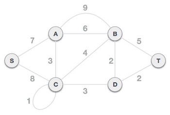
Step 1 - Remove all loops and Parallel Edges
Remove all loops and parallel edges from the given graph.
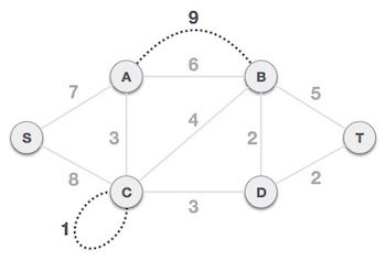
In case of parallel edges, keep the one which has the least cost associated and remove all others.
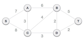
Step 2 - Arrange all edges in their increasing order of weight
The next step is to create a set of edges and weight, and arrange them in an ascending order of weightage (cost).

Step 3 - Add the edge which has the least weightage
Now we start adding edges to the graph beginning from the one which has the least weight. Throughout, we shall keep checking that the spanning properties remain intact. In case, by adding one edge, the spanning tree property does not hold then we shall consider not to include the edge in the graph.
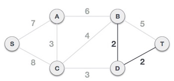
The least cost is 2 and edges involved are B,D and D,T. We add them. Adding them does not violate spanning tree properties, so we continue to our next edge selection.
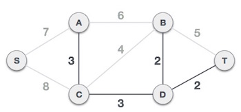
Next cost is 3, and associated edges are A,C and C,D. We add them again −
Next cost in the table is 4, and we observe that adding it will create a circuit in the graph. −
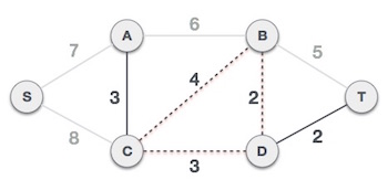
We ignore it. In the process we shall ignore/avoid all edges that create a circuit.
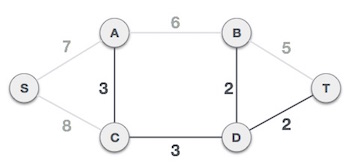
We observe that edges with cost 5 and 6 also create circuits. We ignore them and move on.
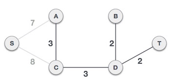
Now we are left with only one node to be added. Between the two least cost edges available 7 and 8, we shall add the edge with cost 7.
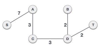
By adding edge S,A we have included all the nodes of the graph and we now have minimum cost spanning tree.
Q-13) Explain indexed file organization.
An indexed file contains records ordered by a record key. A record key uniquely identifies a record and determines the sequence in which it is accessed with respect to other records.
Each record contains a field that contains the record key. A record key for a record might be, for example, an employee number or an invoice number.
An indexed file can also use alternate indexes, that is, record keys that let you access the file using a different logical arrangement of the records. For example, you could access a file through employee department rather than through employee number.
The possible record transmission (access) modes for indexed files are sequential, random, or dynamic. When indexed files are read or written sequentially, the sequence is that of the key values.
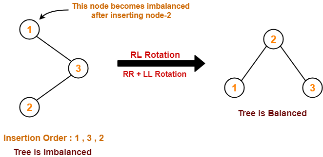
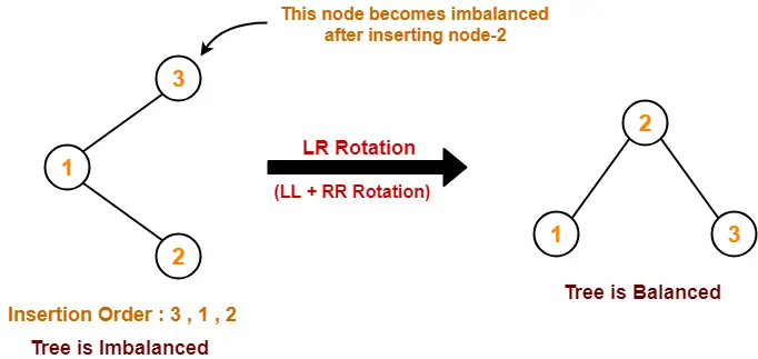
Q-14)Explain rotation rules for AVL tree.
The balance factor of a node is the difference in the heights of the left and right subtrees. The balance factor of every node in the AVL tree should be either +1, 0 or -1.
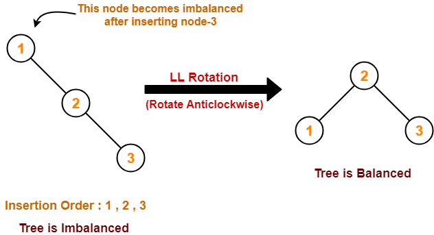
- Left Rotation (LL Rotation)
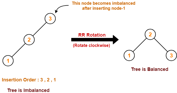
- Right Rotation (RR Rotation)
- Left-Right Rotation (LR Rotation)
- Right-Left Rotation (RL Rotation)
Left Rotation :
Right Rotation :
Left-Right Rotation :
Right-Left Rotation :
